Optimal control problem 2
Conway and K. M. Larson : Collocation Versus Differential Inclusion in Direct Optimization
Use single shooting for transcription
[1]:
import simulatetraj as a
import casadi as cs
import matplotlib.pyplot as plt
define the integrator
integrator grid and transcription grid will match for single shooting
[2]:
sym_dict=a.get_symbols(n_x=2,n_u=1,n_p=0,N=50,cs_type=cs.SX)
x=sym_dict['x']
u=sym_dict['u']
f=cs.vertcat(x[1],-x[1]+u)
_=a.scale_ode(sym_dict=sym_dict,f=f)
_=a.integrator(sym_dict=sym_dict,options=['rk',{}])
[3]:
nlp=cs.Opti()
X0=nlp.variable(sym_dict['n_x'],1)
U =nlp.variable(sym_dict['n_u'],sym_dict['N'])
obj=cs.sumsqr(U)*2/sym_dict['N']

x0=cs.DM([0,0])
a.simulate(sym_dict=sym_dict,t0=0,tf=2,x0=x0,u=U)
X=sym_dict['x_res']

nlp.minimize(obj)
nlp.subject_to(X0-x0==0)
nlp.subject_to(cs.horzcat(1,-2.694528)@X[:,-1]+1.155356==0)
nlp.solver('ipopt')
nlp.set_initial(U,cs.np.linspace(0,1,sym_dict['N']))
sol=nlp.solve()
obj_val=sol.value(nlp.f)
print(f'Objective value: Paper - 0.577678 | code - {obj_val}')
******************************************************************************
This program contains Ipopt, a library for large-scale nonlinear optimization.
 Ipopt is released as open source code under the Eclipse Public License (EPL).
         For more information visit https://github.com/coin-or/Ipopt
******************************************************************************

This is Ipopt version 3.14.11, running with linear solver MUMPS 5.4.1.

Number of nonzeros in equality constraint Jacobian...:       52
Number of nonzeros in inequality constraint Jacobian.:        0
Number of nonzeros in Lagrangian Hessian.............:       50

Total number of variables............................:       52
                     variables with only lower bounds:        0
                variables with lower and upper bounds:        0
                     variables with only upper bounds:        0
Total number of equality constraints.................:        3
Total number of inequality constraints...............:        0
        inequality constraints with only lower bounds:        0
   inequality constraints with lower and upper bounds:        0
        inequality constraints with only upper bounds:        0

iter    objective    inf_pr   inf_du lg(mu)  ||d||  lg(rg) alpha_du alpha_pr  ls
   0  6.7346939e-01 4.81e-02 2.75e-02  -1.0 0.00e+00    -  0.00e+00 0.00e+00   0
   1  5.7790126e-01 4.44e-16 1.39e-17  -2.5 3.43e-01    -  1.00e+00 1.00e+00f  1

Number of Iterations....: 1

                                   (scaled)                 (unscaled)
Objective...............:   5.7790126446789747e-01    5.7790126446789747e-01
Dual infeasibility......:   1.3877787807814457e-17    1.3877787807814457e-17
Constraint violation....:   4.4408920985006262e-16    4.4408920985006262e-16
Variable bound violation:   0.0000000000000000e+00    0.0000000000000000e+00
Complementarity.........:   0.0000000000000000e+00    0.0000000000000000e+00
Overall NLP error.......:   4.4408920985006262e-16    4.4408920985006262e-16


Number of objective function evaluations             = 2
Number of objective gradient evaluations             = 2
Number of equality constraint evaluations            = 2
Number of inequality constraint evaluations          = 0
Number of equality constraint Jacobian evaluations   = 2
Number of inequality constraint Jacobian evaluations = 0
Number of Lagrangian Hessian evaluations             = 1
Total seconds in IPOPT                               = 0.005

EXIT: Optimal Solution Found.
      solver  :   t_proc      (avg)   t_wall      (avg)    n_eval
       nlp_f  |        0 (       0)   3.00us (  1.50us)         2
       nlp_g  |        0 (       0) 184.00us ( 92.00us)         2
  nlp_grad_f  |        0 (       0)  29.00us (  9.67us)         3
  nlp_hess_l  |   1.00ms (  1.00ms) 878.00us (878.00us)         1
   nlp_jac_g  |   1.00ms (333.33us)   1.19ms (396.33us)         3
       total  |   9.00ms (  9.00ms)   5.84ms (  5.84ms)         1
Objective value: Paper - 0.577678 | code - 0.5779012644678975
plot results
[4]:
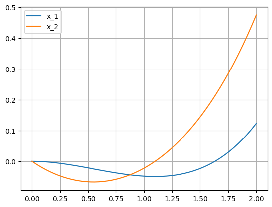
plt.figure()
plt.plot(cs.np.linspace(0,2,50+1),sol.value(X[0,:]).flatten(),label='x_1')
plt.plot(cs.np.linspace(0,2,50+1),sol.value(X[1,:]).flatten(),label='x_2')
plt.legend()
plt.grid(True)
plt.show()
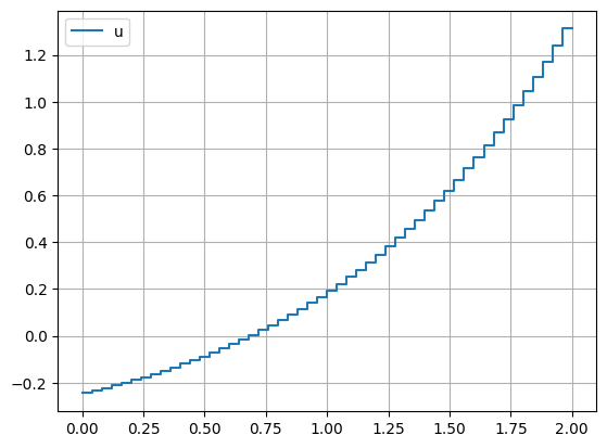
plt.figure()
plt.step(cs.np.linspace(0,2,50+1),cs.np.hstack((cs.np.nan,sol.value(U))),label='u')
plt.legend()
plt.grid(True)
plt.show()
Note that the single shooting method is not robust and may be prone to failure. Multiple shooting methods are recommended.